Matplotlib

---

Ressources:

• Matplotlib

Beyond Matplotlib

• Seaborn - Statistical data visualization
• Cartopy - Geospatial data processing
• yt - Volumetric data visualization
• mpld3 - Bringing Matplotlib to the browser
• Datashader - Large data processing pipeline
• plotnine - A grammar of graphics for Python

And probably much more … If you want to promote a library you are using yourself, feel free to comment and let me know.

Note

Use one data set to set some examples

---

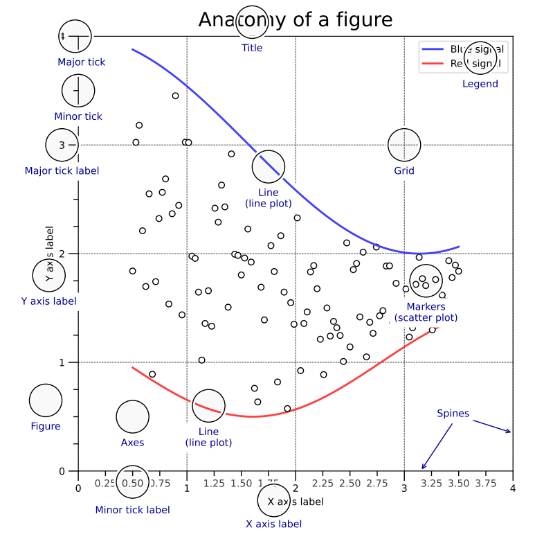
Introduction

import numpy as np
import matplotlib as mpl
import matplotlib.pyplot as plt

X = np.linspace(0, 2*np.pi, 100)
Y = np.cos(X)

fig, ax = plt.subplots()
ax.plot(X, Y, color=’green’)

fig.savefig(“figure.pdf”)
fig.show()

Explanation

Just copy and paste this cell into your Jupyter Notebook editor and run the cell

Voila

You have just created your first plot, Congratulations

Now lets have a look at …

Anatomy of a figure

Fig. 30 source

Plot

» Types

Basic

Fig. 31 source

Advanced

Fig. 32 source

» Styles

Explanation

plt.style.use(style)

Fig. 33 source

Markers

Fig. 34 source

Colors

Color names

Fig. 35 source

» Subplots

layout

Fig. 36 source

Animation

import matplotlib.animation as mpla

T = np.linspace(0, 2*np.pi, 100)
S = np.sin(T)

line, = plt.plot(T, S)

def animate(i):
line.set_ydata(np.sin(T+i/50))
anim = mpla.FuncAnimation(

plt.gcf(), animate, interval=5)
plt.show()